Homework 1

Release Date:: 2024/01/22
Due Date:: 2024/01/29 23:59:59
Topic:: Planetary Formation

Instruction

The format of the homework is constructed as the extension of the lecture. In the homework, you will see familiar concepts that we have learned in the lecture and some new concepts that we have not discussed formally in the lectures. Some problems require single variable calculus including differentiation and integration. You can use any programming language to solve the problems but Python is recommended. Python has a rich set of libraries for scientific computing and visualization. You can use numpy for numerical computation and matplotlib for visualization. The sympy library can be useful for symbolic computation.

You are encouraged to work on the homework with your classmates. However, you must write your own code and submit your own homework assignment. You are not allowed to copy and paste the code from your classmates. You can consult AI tools such as ChatGPT but you must make sure the code is working and produces the correct results. You are fully responsible for the correctness of your code.

To allow us to grade your homework, you must submit both your calculation code and the written answers to Canvas in a combined PDF file. You code will be graded based on the style and your written answers will be graded based on the correctness. (You will not be graded on the style for this homework assignment.)

Solar Property Table

Property	Value
Mass	\(1.989 \times 10^{30}\) kg
Radius	\(6.957 \times 10^8\) m
Luminosity	\(3.828 \times 10^{26}\) W
Effective Temperature	\(5772\) K
Rotation Period	\(25.38\) days

Planet Fact Sheet

Planet	Mass (\(10^{24}\) kg)	Distance from Sun (Au)	Orbital Period (days)
Mercury	0.3285	0.387	88
Venus	4.867	0.723	225
Earth	5.972	1.000	365
Mars	0.6390	1.524	687
Jupiter	1898	5.204	4333
Saturn	568.3	9.582	10756
Uranus	86.8	19.229	30687
Neptune	102.4	30.103	60190

1. (5’) Revisit Laplace’s view of planetary formation

In the 18th century, Laplace proposed a theory of planetary formation. The theory is based on the assumption that the solar system was first immersed in a gaseous of an immense extent and that the planets were formed by the condensation of the gaseous atmosphere. Laplace further postulated that the planets were formed at the successive limits of the gaseous atmosphere when the atmosphere contracted.

From a historical perspective, surmise why Laplace proposed this theory. What kind of observations or facts did Laplace have in mind when he proposed this theory? Did Laplace explain the formation of the solar system in a satisfactory way? Can you rebut Laplace’s hypothetical theory using the knowledge in the 18th century?

What do you think is the most important observation or fact that leads to the downfall of Laplace’s theory and the rise of the modern theory of planetary formation?

2. Angular Momentum of the Solar System - Part I

Angular momentum is a conserved quantity in the absence of external torques. Before the solar system was formed, the space was occupied by a cloud of gas and dust, known as the Giant Molecular Cloud (GMC). The GMC was rotating and the angular momentum of the GMC was conserved. As the GMC collapsed, the angular momentum was conserved and the rotation rate of the GMC increased because the GMC became smaller. The GMC eventually collapsed into a disk and the disk eventually formed the Sun and the planets. The angular momentum distribution of the solar system gives clues to the formation of the solar system.

This problem is to calculate the angular momentum of the solar system objects and understand the angular momentum distribution of the solar system.

The biggest object in the solar system is the Sun. The Sun has a mass of \(M_\odot = 1.989 \times 10^{30}\) kg and a radius of \(R_\odot = 6.957 \times 10^8\) m. The Sun rotates with a period of \(P_\odot = 25.38\) days. In the first part of the problem, you will calculate the angular momentum contained in the Sun. In the second part of the problem, you will calculate the angular momentum of the planets in the solar system.

To calculate the angular momentum of the Sun, we need to calculate the angular momentum of every piece of the Sun and sum them up. The Sun is a sphere and we can divide the Sun into many small pieces. The angular momentum of a small piece of the Sun is given by

\[\mathrm{d} L = r_{\perp} v \mathrm{d} m,\]

where \(r_{\perp}\) is the distance perpendicular to the rotation axis, \(v\) is the velocity, and \(\mathrm{d} m\) is the mass of the small piece. The \(\mathrm{d}\) symbol stands for an infinitesimal quantity and we will use this notation throughout the lectures and the homework assignments. As a result, the symbol \(\mathrm{d} L\) stands for the infinitesimal angular momentum of a small piece of the Sun and the symbol \(\mathrm{d} m\) stands for the infinitesimal mass of a small piece of the Sun.

For a spherical body that rotates around a fixed axis, the velocity of a small piece of the body is given by:

\[v = \Omega r_{\perp},\]

where \(\Omega\) is called the angular velocity of the rotation.

(a) (1’) Calculate the angular velocity of the Sun in rad/s.

You can use the Solar Property Table to find the rotation period of the Sun. Then, you can calculate the angular velocity of the Sun based on the rotation period.

The infinitesimal mass of a small piece of the Sun is related to the density \(\rho\) and the volume \(\mathrm{d} V\) of the small piece by:

\[\mathrm{d} m = \rho \mathrm{d} V.\]

We shall simplify the calculation by assuming the Sun is a uniform sphere, i.e., the density of the Sun, \(\rho\) is the same everywhere. Next, we will figure out how to calculate the volume of this small piece in some coordinate system.

We will use the spherical polar coordinate system to describe the position of the small piece. The origin of the coordinate system is at the center of the Sun. The \(z\)-axis is aligned with the rotation axis of the Sun. The \(x\)-axis is in the plane of the Sun’s equator and the \(y\)-axis is perpendicular to the \(x\)-axis and the \(z\)-axis. An illustration of the geometry is shown in the figure below.

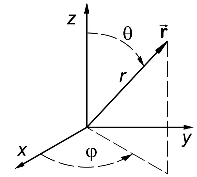
_images/spherical_polar.png — The spherical polar coordinate system

In the spherical polar coordinate system, the position of the small piece is given by \((r, \theta, \phi)\), where \(r\) is the distance from the origin, \(\theta\) is the angle between the \(z\)-axis and the position vector, and \(\phi\) is the angle between the \(x\)-axis and the projection of the position vector onto the \(x\)-\(y\) plane. The volume of the small piece is given by:

\[\mathrm{d} V = r^2 \sin \theta \mathrm{d} r \mathrm{d} \theta \mathrm{d} \phi.\]

The distance perpendicular to the rotation axis is given by:

\[r_{\perp} = r \sin \theta.\]

Now, we can assemble all the pieces together and express the angular momentum of the small piece as:

\[\mathrm{d} L = \Omega \rho r^4 (\sin \theta)^3 \mathrm{d} r \mathrm{d} \theta \mathrm{d} \phi.\]

(b) (1’) Fill in the missing steps in deriving the above equation

Many equations are involved to get the right result. You should convince yourself that the above equation is correct.

The last step is to sum up the angular momentum of all the small pieces of the Sun:

\[L_\odot = \Omega \rho \int_0^{2 \pi} \mathrm{d} \phi \int_0^{R_\odot} r^4 \mathrm{d} r \int_0^{\pi} (\sin \theta)^3 \mathrm{d} \theta\]

It is a multi-dimensional integral but we can simplify that by integrating over one dimension at a time. We will integrate over the \(\phi\) direction first, which yields \(2 \pi\). Then, we will integrate over the \(r\) direction from \(0\) to \(R_\odot\), where \(R_\odot\) is the radius of the Sun. Finally, we will integrate over the \(\theta\) direction from \(0\) to \(\pi\). You can use the approximation that \(\rho\) is a constant.

(c) (2’) Finish the steps in the integration

You should get a result that is a function of three symbols: (1) the density of the Sun, (2) the radius of the Sun, and (3) the angular velocity of the Sun. Do not plug in the numbers yet. Do not feel intimidated by the multi-dimensional integral. You do not live in the stone age. Feel free to use any online integral calculator to help you with the integration. For example, I use Wolfram Alpha quite often to help me with complex integrals. You are allowed to use online tools in your midterm exam. The homework does not test your ability to do integrals. It trains your ability to understand the physics and can use the necessary tools to solve the problem.

You can use the Solar Property Table of the Sun to find the radius of the Sun and the rotation period of the Sun. However, you cannot get the density from the Solar Property Table. This is because the density of the Sun normally varies with the depth.

To make the calculation easier, we have assumed that the density of the Sun is a constant. This is an approximation in the context of solving this problem. In reality, we make various approximations to make a problem solvable. No problem can be solved without making any approximation or qualification. The key is to make the right and reasonable approximation.

Suppose that the density of the Sun is \(\rho_\odot = 1.35 \times 10^3\) kg/m^3.

(d) (1’) Calculate the angular momentum of the Sun

The key to get this problem right is to mind the units. I suggest converting all the units to SI units before plugging in the numbers. Carry all units throughout the calculation and make sure that your final result should have the unit of kg m^2/s.

(e) (bonus 1’) Explain why the density of the Sun is \(\rho_\odot = 1.35 \times 10^3\) kg/m^3

There is a reason why I choose this number. Since we know the mass and the radius of the Sun from the Solar Property Table, we should be able calculate the density of the Sun. The process is similar to the calculation of the angular momentum of the Sun. If you can get this number, you are awarded one bonus point toward this problem, meaning that you can get 6/5 for this problem.

3. Minimum Mass Solar Nebula

The Minimum Mass Solar Nebula (MMSN) is a model of the protoplanetary disk around the Sun before the formation of the planets. The MMSN model is constructed by assuming that the protoplanetary disk has the minimum mass required to form the planets in the solar system. The MMSN model is a useful reference for understanding the formation of the solar system and identify anomalies.

The problem asks you to reproduce the MMSN model and draft a plot of the surface density of the MMSN as a function of the distance from the Sun. You will need the Planet Fact Sheet of the solar system for the density and location of the major planets.

Assuming the following planet formation scenario:

Terrestrial planets like Mercury, Venus, Earth, and Mars only retain the refractory materials in the protoplanetary disk. The mass fraction of the refractory materials among all available materials is about 0.3%.

The ice giants like Uranus and Neptune retain both refractory and volatiles in the protoplanetary disk. The mass fraction of the refractory and volatile materials among all available materials is about 5%.

The gas giants like Jupiter and Saturn retain about 20% of the available materials in the protoplanetary disk including refractory, volatile, and gaseous materials. The remaining 80% of the available materials are blown away by the solar wind.

(a) (1’) Divide the protoplanetary disk into concentric, disjoint annulus.

Each annulus should have a width, covering a region of the protoplanetary disk between an inner radius and an outer radius. Each annulus is associated with exactly one planet that represents the formation region of the planet in the disk.

The annuli must be disjoint and completely covers the entire protoplanetary disk from 0.1 AU to 50 AU.

You can make the judgement call to choose the boundaries of the annuli. Design eight annuli that cover the eight major planets in the solar system. You may use the numpy.logspace function to generate the logarithmically spaced values or numpy.linspace function to generate the linearly spaced values.

Report the boundaries and the area of the annuli in a table.

(b) (2’) Calculate the mass of each annulus

Use the method described in class to calculate the mass of each annulus in the protoplanetary disk. Report the mass of each annulus in a table.

(c) (2’) Make a plot of the surface density of the MMSN as a function of the distance from the Sun.

The surface density of the MMSN is the mass of each annulus divided by the area of the annulus. Use the matplotlib.pyplot.step function to draw “stairs”. Use the matplotlib.pyplot.xlabel and matplotlib.pyplot.ylabel functions to label the x-axis and y-axis, respectively. Use the matplotlib.pyplot.xscale and matplotlib.pyplot.yscale functions to set the scale of the x-axis and y-axis to both be logarithmic. Use the matplotlib.pyplot.savefig function to save the figure.

4. N-body simulation with Python

N-body simulation is a computational method to study the motion of a group of objects interacting with each other under a mutual force. The force can be gravitational force, electrostatic force, or any other contact force. N-body simulation is widely used in astrophysics to study the formation of Stars and planets. For performance reasons, N-body simulation is usually implemented in a compiled language such as C or Fortran. However, for the purpose of learning, we will use a N-body simulation code written in Python to have a taste of how N-body simulation works.

The model we will use in this problem is written by Philip Mocz, a computational physicist at Lawrence Livermore National Lab. The model is publicly available at here.

(a) (1’) Clone the Github repository and download the N-body simulation code

You must first register a GitHub account if you do not have one. Do not download the code as a zip file. You must use git clone to clone the repository. If you have a Mac or Linux computer, you can use the git command directly in the terminal. If you are using Windows, you can either install Windows Subsystem for Linux (WSL) first and use the git command in the terminal or use Visual Studio Code to clone the repository.

(b) (1’) Run the N-body simulation code

The N-body simulation code is written in Python3. You must have Python3 installed on your computer to run the code. You can use the python3 command directly in the terminal if you have a Mac or Linux computer. If you are using Windows, you can use the python3 command in the terminal provided by WSL.

If you have Jupyter Notebook installed, you can also run the code in a Jupyter Notebook. Take screenshots of the output of the code and include them in your report.

(c) (1’) Read the code and understand how it works

The code is well documented. You should be able to understand how the code works by reading the comments in the code. Write a short paragraph to explain how the code works.

(d) (1’) Change the initial conditions of the simulation to simulate the Sun-Earth system

Find out where the initial conditions are set in the code. Change the initial conditions to be solar system like. You can use the Planet Fact Sheet of the solar system to find out various properties of the solar system.

You may follow the following steps to change the initial conditions. Make sure that the code still works after each step. You may need to change the time step and the total time to make the simulation work. You may need to adjust the limits of the plot to make the plot look nice. Gravitational constant was set to be 1 in the code. You may need to change it to be the real value.

Change the number of particles to 2. They represent 2 planets.

Change the mass of the particles to be the mass of the Sun and the mass of the Earth.

Change the initial position of the particles to be the position of the Sun and the Earth.

Change the initial velocity of one particle to be the orbital velocity of Earth. You can use the orbital period to calculate the orbital velocity.

Change the time step to be 1 day.

Change the total time to be 1 year.

Run the simulation and summarize the results.

(e) (1’) Change the initial conditions of the simulation to be solar system like

Add more particles to the simulation to represent more planets.

Adjust the limits of the plot to make the plot look nice.

Run the simulation and summarize the results.